In Heroes of Might and Magic: Olden Era, armies fight on a hexagonal battlefield. To turn a screenshot into useful cell positions, a program first needs to locate that grid. Creatures obscure its edges, terrain introduces extra lines, and the angled camera distorts the hexagons.
The useful shortcut is that the grid’s geometry is already known. Calibrate its projection once, then make small adjustments around that saved position. This experiment outputs cell centers and outlines, but its three inspected test images still have a median vertex error of 18.8 pixels. The close-ups below explain both how the fit works and why its score can be misleading.
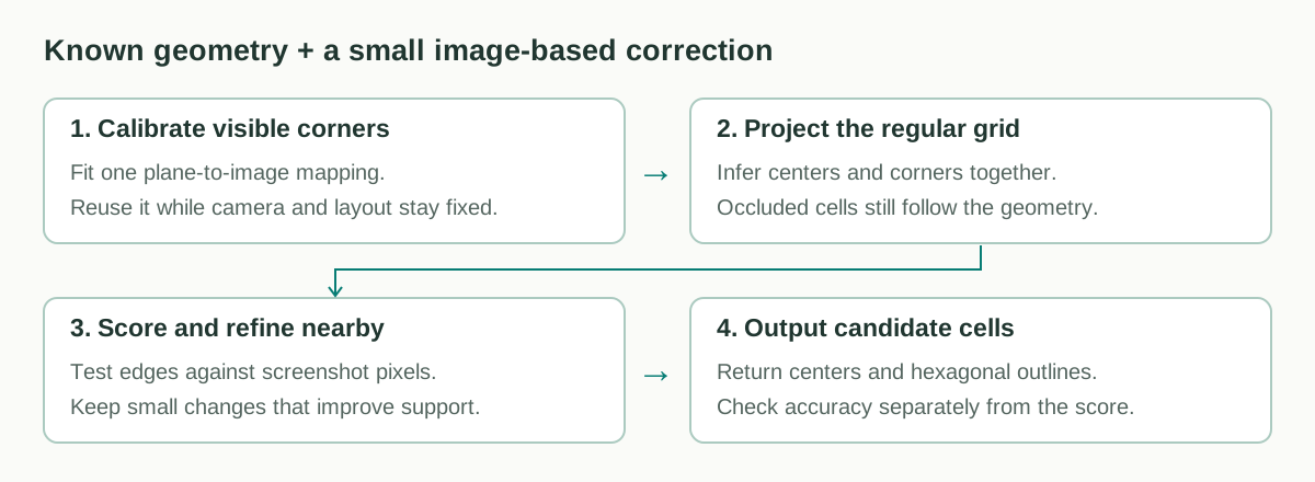
Figure 1. One shared projection describes the whole grid. The screenshot supplies evidence for a small correction around the calibration.
1. Start from a calibrated grid
Imagine a transparent sheet of regular hexagons laid over the screenshot. Adjust its size, position, and perspective until the corners match. Because neighboring cells share the same geometry, a few known cells constrain the rest of the sheet—even where creatures cover the seams.
The plane-to-image mapping is called a homography. It can describe sideways tilt and spacing that changes with depth. We fit it using 36 visible corners from six cells, distributed across one calibration image.

Figure 2. Calibration image. The magenta points were placed by visual inspection of source pixels, without snapping them to a predicted grid. All 36 corners contribute to the initial mapping.
Once camera position, zoom, image resolution, and screenshot crop stay fixed, the grid should remain near this calibrated placement. Each new screenshot starts from the same saved mapping. The search makes a small correction; it does not start over across the full image or accumulate corrections from earlier frames.
One confirmed position can anchor translation after scale, orientation, and perspective are known. One point alone cannot determine all those properties. The current implementation permits small adjustments to the full mapping rather than locking one corner in place.
The input is a 1920 × 1078 screenshot. The output is each candidate cell’s center, six vertices, and relative grid coordinates. These do not establish the true board boundary, occupancy, or whether a unit can stand in a cell.

Figure 3. Development image. These 17 points measure the fit after the image-based search; they do not guide it. The median vertex error on this image is 8.5 pixels.
The full set contains one calibration image, two development images, and three test images from six different videos, with 106 reference points. The development set selected the refinement method. The labels are Codex visual annotations awaiting human review, with uncertainty around blurred seams, occlusion, and the cursor. All examples here have been inspected; they are not fresh validation on unseen videos.
2. What does it mean for a proposed edge to score well?
The geometry component generates a regular grid. The image component asks whether its proposed edges follow visible lines. The search component adjusts the grid and keeps placements with a better overall score.
First, convert the screenshot to grayscale and smooth small variations with a Gaussian blur. Then Sobel derivatives measure brightness changes in two directions. Combining them produces an edge-magnitude image: strong changes look bright. A bright rock or creature outline appears here just as a grid seam does.
For one proposed edge, the program takes seven samples along its interior. At each sample it asks two questions:
- Does brightness change across this line? Check the gradient perpendicular to the proposed edge, at the center and up to 2 pixels on either side. This contributes at most 0.55.
- Is there a bright or dark line here? Compare the center brightness with the average brightness 5 pixels to either side. This contributes at most 0.45.
Both contributions are clipped before addition, so one sample can score at most 1. Their average becomes the edge score. Coordinates between pixels are read with bilinear interpolation.
Next, average valid edge scores inside each of twelve spatial regions, and give the regions equal weight. This region-balanced objective encourages support across the image. It is the number the search maximizes.
The score means “line-like brightness structure near the prediction.” It is not a probability that the grid is correct. The next three examples make that distinction visible.
3. Three close-ups: high, low, and misleading scores
Each figure follows the same reading order: source pixels → Sobel magnitude → proposed line and sample positions → seven numerical responses. Every panel uses the same crop. Cyan marks the prediction; short orange strokes cross it in the sampling direction. Teal bars show gradient contributions and orange bars show bright/dark-line contributions.
These three candidates come from the same red-terrain screenshot, at the final fitted position. They share the same normalization scale. They were selected afterward to explain the score, not to estimate how frequently each situation occurs. Click any figure to inspect it full screen.
A visible terrain seam: 0.861
The proposed line runs along a visible seam. Sobel finds strong brightness changes nearby, and most sample positions receive substantial contributions. Four of the seven samples reach the cap of 1. The edge’s mean is 0.861.
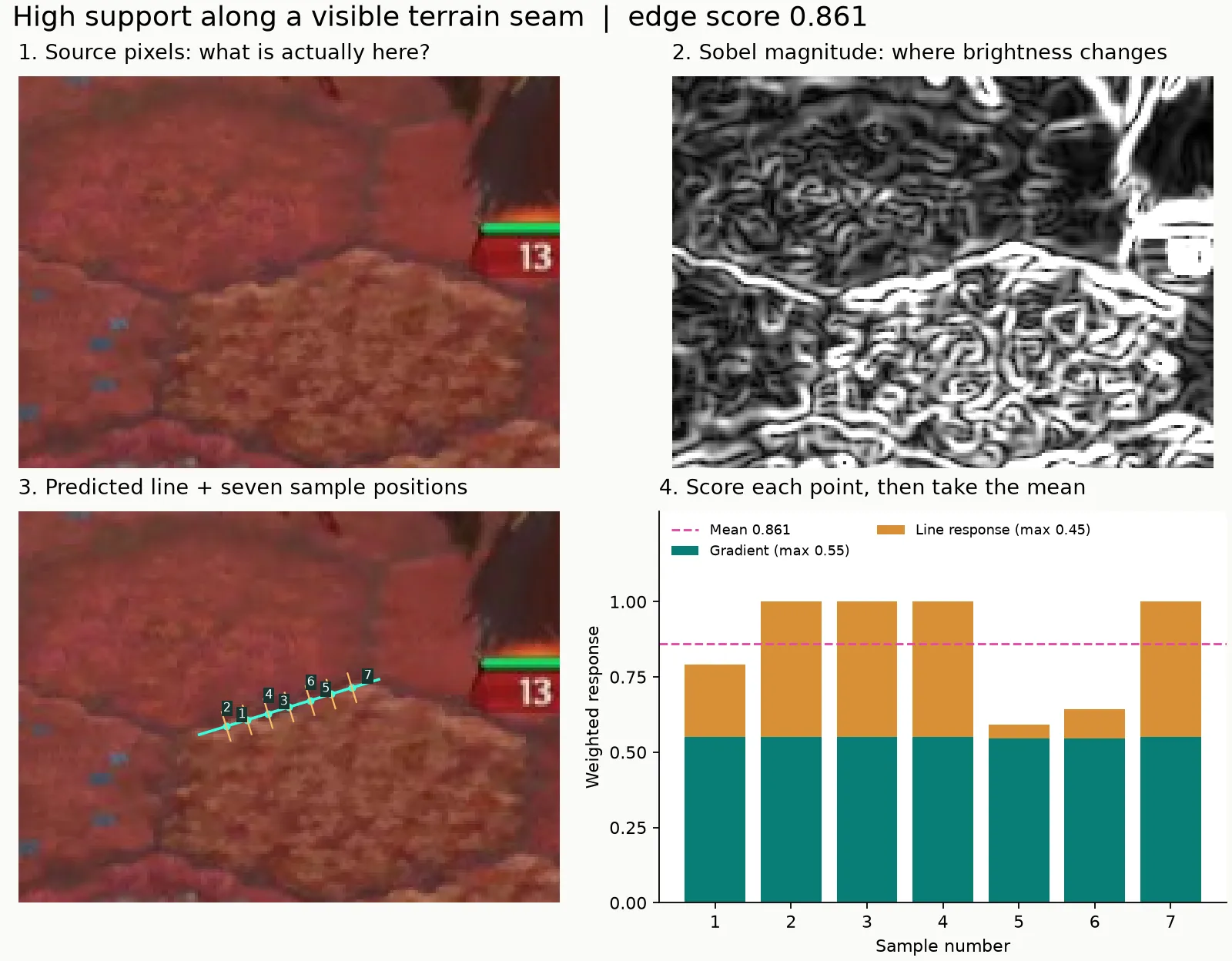
Figure 4. High support. The seven bars correspond to the seven numbered points. This is the kind of evidence we want a proposed grid edge to collect.
A line across nearly uniform ground: 0.060
This prediction crosses a comparatively flat patch beside a rock. The rock creates strong edges elsewhere in the crop, but the seven samples do not follow them. Both scoring terms stay small, producing a mean of 0.060.
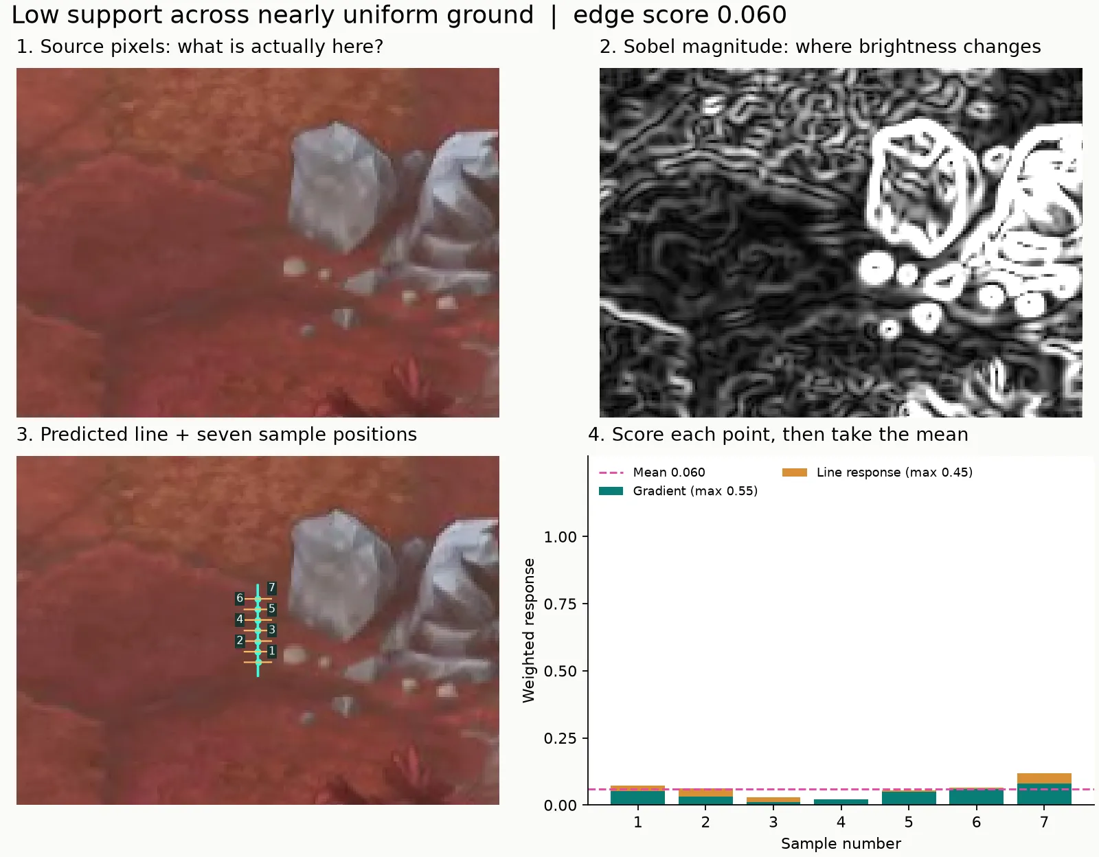
Figure 5. Low support. Strong edges somewhere in the crop are insufficient: the response must occur near the proposed line and in a useful direction.
Creature texture can score even higher: 0.896
Here the line crosses a creature’s body. The nearby texture supplies strong gradients and contrast, giving the candidate 0.896—higher than the visible seam in the first example. We cannot observe a ground seam through the creature, so this score does not verify the predicted edge’s location.
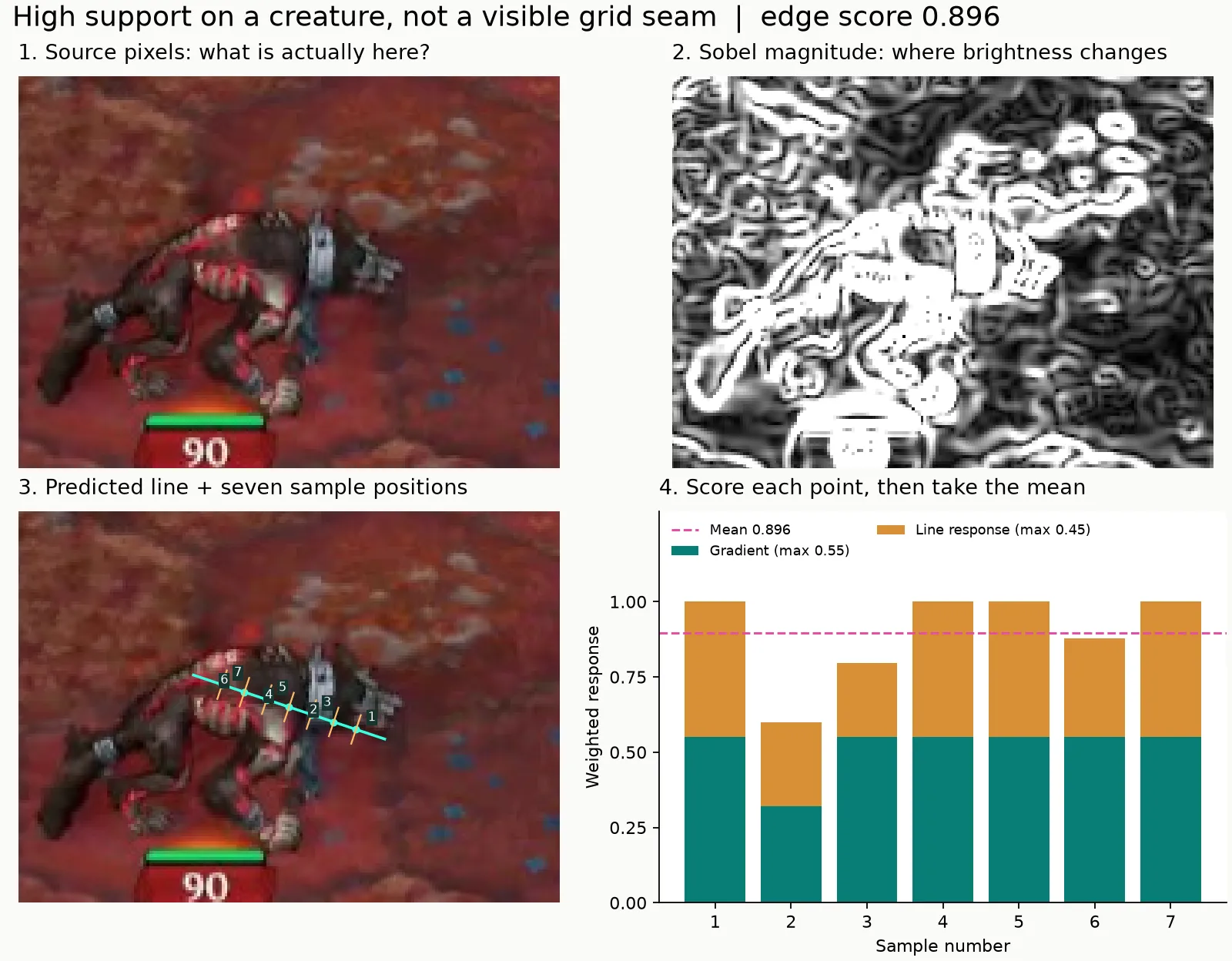
Figure 6. Misleading support. The score sees brightness structure without knowing whether it belongs to the ground grid or the foreground creature.
Clipping limits extreme responses, and spatial averaging reduces one patch’s influence. Neither operation tells the program what a creature is. That explains why maximizing the score can still move a grid in the wrong direction.
4. Watch a fit move, one accepted update at a time
The search begins with the saved calibration. It tries a few nearby values for one parameter, keeps a better-scoring value, and moves on to the next parameter. It repeats with finer steps. This is a bounded coordinate search.
The parameters control translation, scale, rotation, and shear. Their small affine correction is applied after the calibrated projection:
final mapping = small screen-space correction × saved calibration
In particular, translation is limited to ±18 pixels and rotation to ±0.6°. This works only when the initial mapping is already close. It cannot recover a large camera change.
A corner that moves closer to its reference
The next crop is from the snow development image. The source pixels and Sobel image remain fixed throughout the search. Only the projected grid moves.
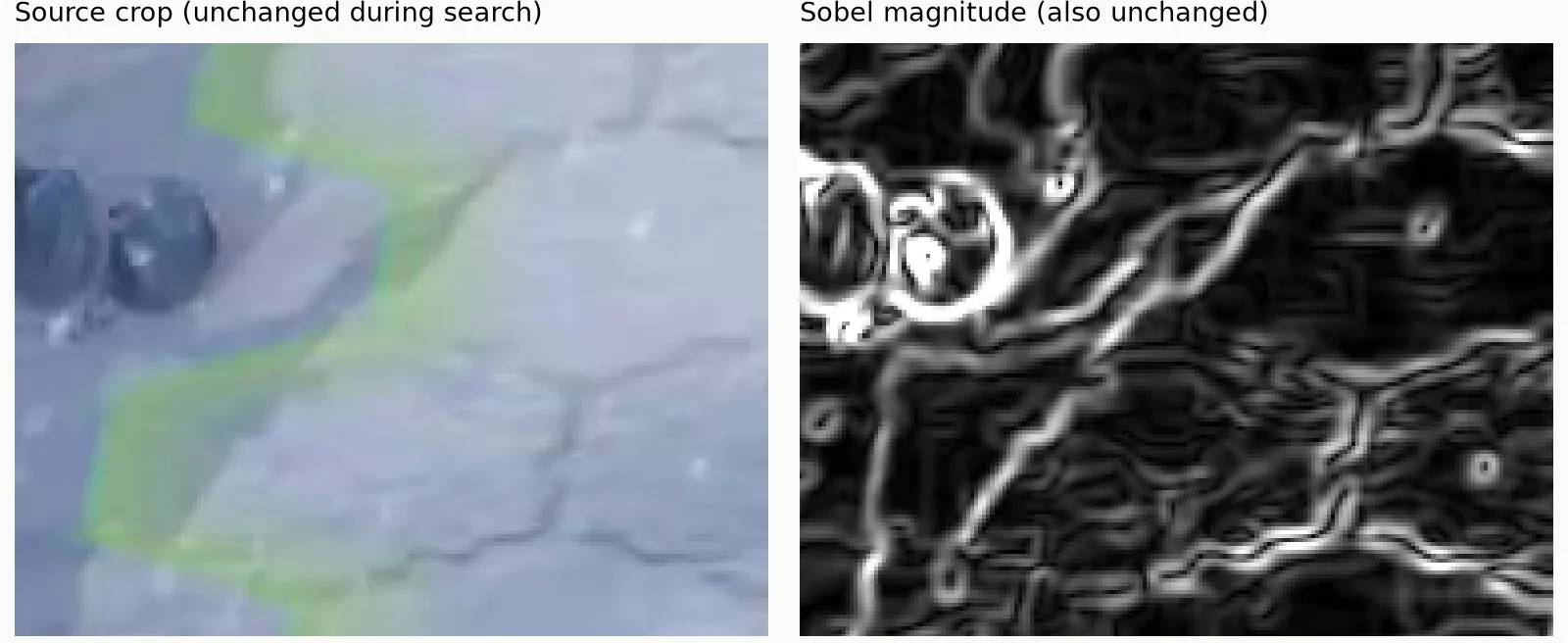
Figure 7. The input evidence. The moving prediction is drawn separately below, so it cannot be mistaken for an edge detected in the source image.
In the next figures, the magenta cross is one pre-existing manual reference; the white circle is the nearest predicted vertex. The short magenta segment measures their separation. This reference is used only to explain the result after the search, never as a search target.
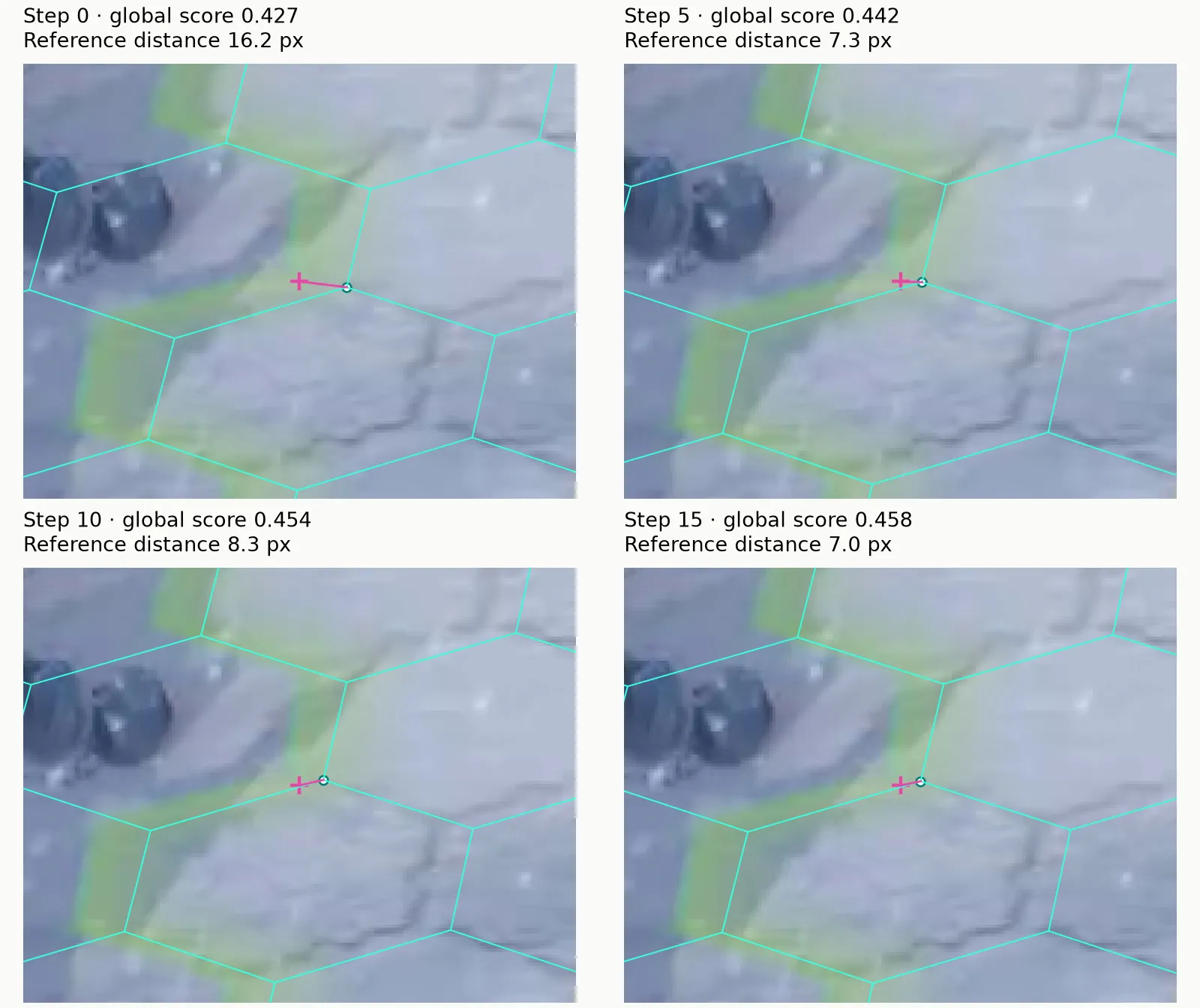
Figure 8. Selected snapshots from the actual search: updates 0, 5, 10, and 15. The corner ends closer, from 16.2 to 7.0 pixels away, but improvement is not monotonic.
Global score 0.427 · reference distance 16.2 px
Using the saved calibration.
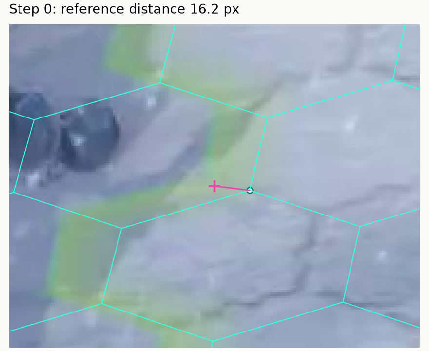
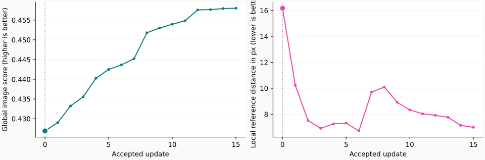
The left curve plots the global image score, which the algorithm can see. The right curve plots distance to this one manual reference, which it cannot see during search. The highlighted points follow the slider. These are discrete recorded updates joined by lines, not a fitted trend or a guarantee of convergence.
A higher score can also move a corner farther away
The red-terrain test image gives a useful counterexample. Its selected-cell outline is bright, yet the final grid still misses the annotated corner. The global score rises from 0.405 to 0.414, while this corner’s reference distance increases from 15.2 to 22.2 pixels.
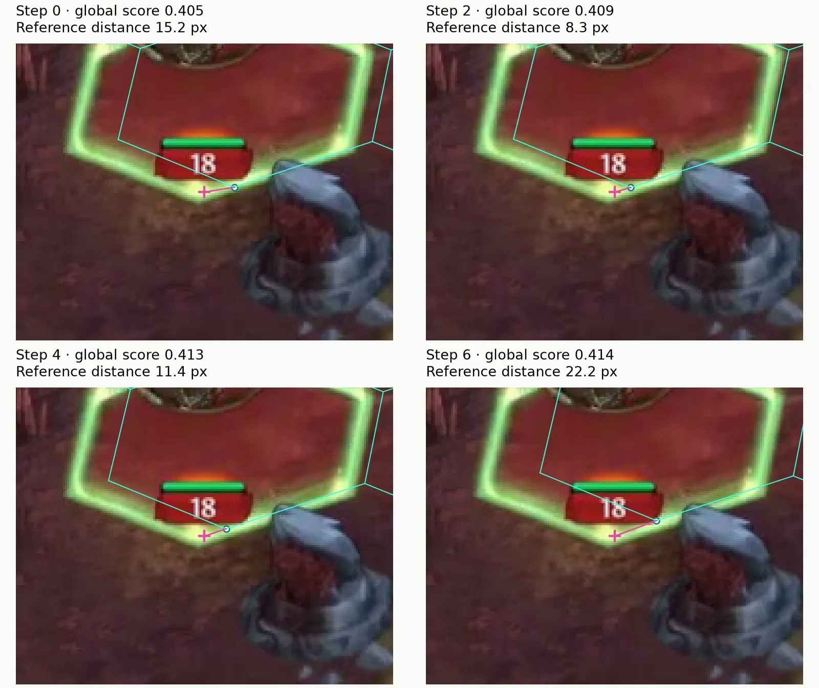
Figure 10. Updates 0, 2, 4, and 6 from one run. A fit can briefly approach this corner and then move away while improving support elsewhere.
Global score 0.405 · reference distance 15.2 px
Using the saved calibration.
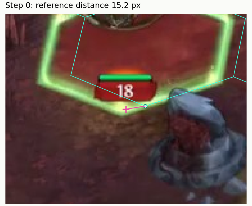
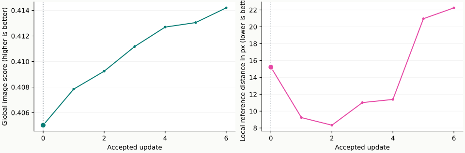
These two crops are teaching examples, not separate accuracy benchmarks. They explain why we must measure geometric error independently of the score we optimize. A more reliable calibration and better discrimination between seams and foreground texture are still needed.
5. Inspect the full computer-vision pipeline
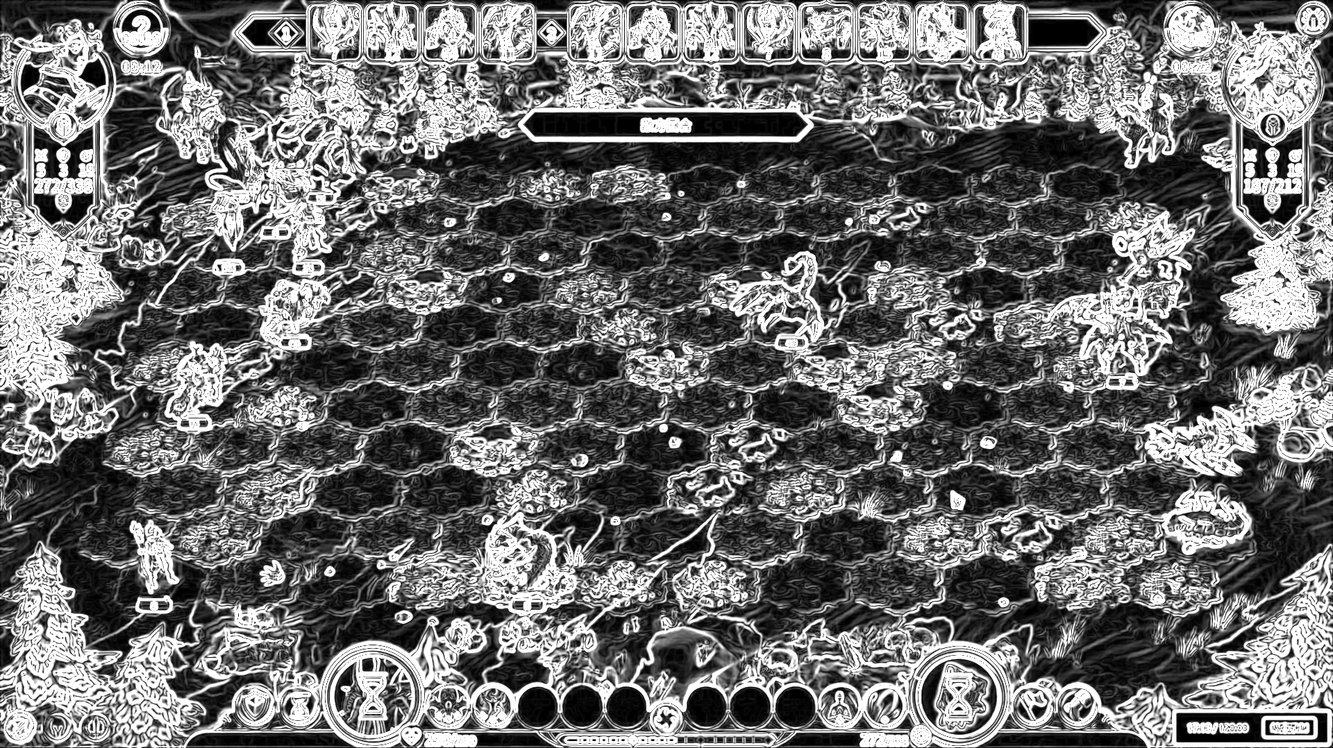
The close-ups explain the mechanism. This explorer puts it back into the complete battlefield: grayscale, blur, both Sobel derivatives, the ideal grid, its initial projection, scoring regions, edge support, and the final fit. All intermediate arrays and scores come from the same implementation that produced the results.
The detail crop stays fixed across stages. The combined Sobel magnitude is a visualization; the score uses the derivative component perpendicular to each proposed edge. Selecting another battlefield changes the evidence, not the algorithm.
Display √(Gx² + Gy²), normalized by this image’s gradient scale and clipped to 0–1. This helps visualize edges; actual grid scoring uses the gradient component perpendicular to each candidate edge.
6. Three complete test outputs
The following images show only the algorithm’s predicted grid on the original screenshots. Cyan lines over creatures and obstacles are inferred from regular geometry. They do not establish that those cells are visible or traversable.
Snow battlefield
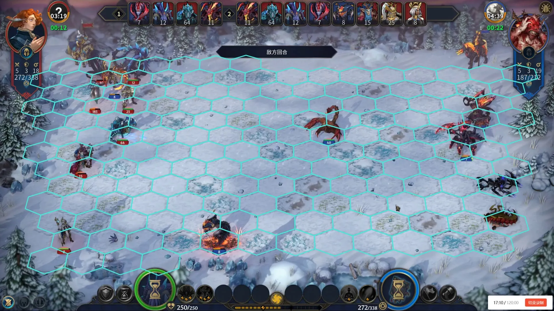
Figure 13. Snow test image: median nearest-vertex error 19.7 pixels over 18 reference points.
Red-terrain battlefield
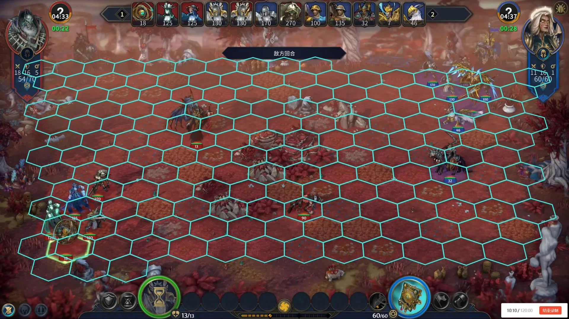
Figure 14. Red-terrain test image: median nearest-vertex error 18.5 pixels over 17 reference points.
Lava battlefield
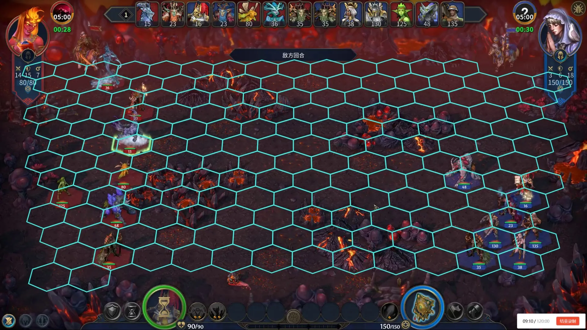
Figure 15. Lava test image: median nearest-vertex error 12.0 pixels over five points on one selected-cell outline. This local measurement cannot establish accuracy across the whole battlefield.
Nearest-vertex error measures the distance from each reference point to the closest predicted corner. Pooling all three test images gives:
| Measurement | Observed result |
|---|---|
| Median vertex error | 18.8 px |
| 95th-percentile error | 33.8 px |
| Reference points within 8 px | 6 / 40 |
Visible offsets remain. All three images also pass the current heuristic confidence check despite these errors, so that check does not reliably identify a bad fit. The measurements assess sparse alignment, not cell occupancy, absolute cell numbering, or every part of the board.
7. What to take away
Known grid geometry makes calibration a useful starting point. A shared projection reconstructs the candidate lattice, and image evidence can refine it within a small neighborhood. But a high edge score means that brightness structure supports a line; it does not tell us whether that line belongs to the battlefield grid.
The current experiment produces full grids automatically, yet its median test error remains 18.8 pixels. The practical next steps are to review the calibration, reduce foreground and texture contamination in scoring, and evaluate on new videos. The local examples show why those changes matter: the search follows its score, while correctness needs an independent check.
8. Algorithm references
Hover or focus a dotted term for a short explanation; click or tap it to jump here. The OpenCV links explain standard operations. The weights and search limits describe this experiment’s implementation.
Homography: mapping a plane into an image
A 3 × 3 matrix with eight independent parameters maps an ideal grid point into the screenshot. Multiply its homogeneous coordinate [u, v, 1] by the matrix, then divide the first two outputs by the third. That division allows perspective distortion. See OpenCV’s homography tutorial.
This experiment calls cv2.findHomography(..., method=0) on all 36 correspondences, without automatic outlier rejection. A general homography needs at least four point pairs in a nondegenerate arrangement. Well-spread, consistent references constrain the fit across the image. The saved mapping is reused in every frame.
Gaussian blur: reducing fine variations
A Gaussian filter averages neighboring pixels with more weight on nearby pixels. This softens noise and fine texture before derivatives amplify them. Here, grayscale is scaled to 0–1 and blurred with σ = 1.2 pixels. Excessive blur would also erase useful seams. See OpenCV’s smoothing tutorial.
Sobel and directional edge response
Sobel estimates horizontal and vertical brightness derivatives, Gx and Gy. The magnitude √(Gx² + Gy²) shows strong changes in any direction. This implementation uses 3 × 3 kernels and divides each derivative by 8. See OpenCV’s Sobel tutorial.
The display shows absolute values, normalized and clipped to 0–1. Scoring retains signed derivatives and takes their component along an edge’s unit normal n. For each sample p, it combines:
g = max over d = −2, 0, 2 of |gradient(p + d n) · n|
r = |(I(p + 5n) + I(p − 5n)) / 2 − I(p)|
response = 0.55 × clip(g / s, 0, 1)
         + 0.45 × clip(r / (3s), 0, 1)
I is blurred grayscale. The scale s is the 90th percentile of gradient magnitude in a central window, with a floor of 0.008. It is fixed for one image. Seven samples span 15%–85% of an edge’s length, avoiding corner junctions; at least four must be inside the scoring window.
Bilinear interpolation: reading between pixels
Projected coordinates usually fall between pixel centers. Bilinear interpolation estimates their values by blending the four surrounding pixels. The implementation uses cv2.remap with INTER_LINEAR for grayscale and derivative arrays. This reduces jumps caused by rounding; it does not create missing image evidence. See OpenCV’s image-transformation documentation.
Region-balanced scoring: combining local evidence
The scoring window spans 8%–92% of image width and 21.5%–83% of image height. Four columns and three rows divide it into twelve regions. Each edge is assigned by its midpoint. A region averages its valid edges, or receives zero if fewer than five are valid. The mean of all twelve region scores is the global objective.
Each region has equal weight, so one region with many candidate edges does not dominate simply by count. There is no creature or obstacle segmentation in this version.
Affine correction: moving the calibrated grid
An affine transform permits translation, scale, rotation, and shear while preserving straight lines and parallelism in the space where it acts. Here it acts on the already-projected grid in screen coordinates. The final mapping is A × H_calibration.
The linear part of A is rotation × [[scale, shear], [0, scale × sy]], applied around the image center, plus translation. It adjusts placement without refitting a complete perspective model on each image. OpenCV describes affine mappings in its geometric-transformation documentation.
Bounded coordinate search: trying nearby values
The search starts from zero translation, zero rotation, unit scale, and zero shear. It tries seven nearby values for one parameter while holding the others fixed, keeps an improvement, then advances to the next parameter. Three finer search levels each make two passes through the parameters.
Translation is bounded to ±18 pixels in each direction; uniform scale to 0.988–1.012; rotation to ±0.6°; shear to ±0.012; and extra vertical scale to 0.988–1.012. All limits are relative to the saved calibration. Only accepted updates appear in the teaching curves. Reference annotations never enter the search.
Nearest-vertex distance and what it excludes
For each annotated corner, find the closest predicted vertex and measure Euclidean distance in pixels. The median describes the middle error, and the 95th percentile describes the upper tail. The headline aggregate pools 40 test points.
For the two illustrated trajectories, the same logical predicted vertex stays nearest throughout the run. The magenta connector therefore follows its displacement relative to one fixed manual point. These labels remain approximate. Neither this measurement nor a periodic grid match establishes absolute game cell IDs, board extent, occupancy, or traversal rules.
Reproducibility and validation
The experiment lives in perception/experiments/b06_battle-hex-grid-registration/ in the local Olden Era workspace. registration.py computes image evidence and bounded refinement; build_teaching_figures.py renders the cases and trajectories shown here. The teaching figures reuse the saved experiment and verify their final matrices and objective values against its recorded outputs. The article’s image files and interaction data live beside its MDX source in the desktop Blogs project.
The geometry tests check synthetic projection and data-separation contracts. They do not establish real-image accuracy. The real-image measurements and visible failures above are the evidence for that question. No learned model or GPU is required by this grid-fitting code.
Comments